07. cvxpy
cvxpy
What is
cvxpy
?
cvxpy
is a Python package for solving convex optimization problems. It allows you to express the problem in a human-readable way, calls a solver, and unpacks the results.
cvxpy
Example
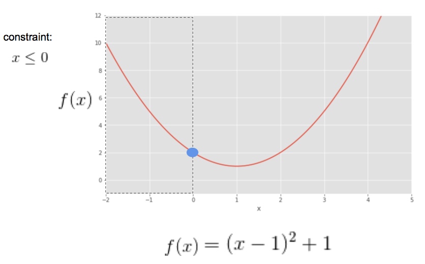
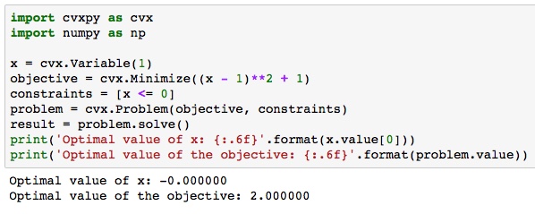
Below, please find an example of the use of
cvxpy
to solve the simple example we referred to in the lectures, optimizing the objective function
(x - 1)^2 +1
subject to the constraint
x \leq 0
.
How to use
cvxpy
Import
: First, you need to import the package:
import cvxpy as cvx
Steps
: Optimization problems involve finding the values of a
variable
that minimize an
objective function
under a set of
constraints
on the range of possible values the variable can take. So we need to use
cvxpy
to declare the
variable
,
objective function
and
constraints
, and then solve the problem.
Optimization variable
: Use
cvx.Variable()
to declare an optimization variable. For portfolio optimization, this will be
\mathbf{x}
, the vector of weights on the assets. Use the argument to declare the size of the variable; e.g.
x = cvx.Variable(2)
declares that
\mathbf{x}
is a vector of length 2. In general, variables can be scalars, vectors, or matrices.
Objective function
: Use
cvx.Minimize()
to declare the objective function. For example, if the objective function is
(\mathbf{x} - \mathbf{y})^2
, you would declare it to be:
objective = cvx.Minimize((x - y)**2)
.
Constraints
: You must specify the problem constraints with a list of expressions. For example, if the constraints are
\mathbf{x} + \mathbf{y} = 1
and
\mathbf{x} - \mathbf{y} \geq 1
you would create the list:
constraints = [x + y == 1, x - y >= 1]
. Equality and inequality constraints are elementwise, whether they involve scalars, vectors, or matrices. For example, together the constraints
0 <= x
and
x <= 1
mean that every entry of
\mathbf{x}
is between 0 and 1. You cannot construct inequalities with < and >. Strict inequalities don’t make sense in a real world setting. Also, you cannot chain constraints together, e.g.,
0 <= x <= 1
or
x == y == 2
.
Quadratic form
: Use
cvx.quad_form()
to create a quadratic form. For example, if you want to minimize portfolio variance, and you have a covariance matrix
\mathbf{P}
, the quantity
cvx.quad_form(x, P)
represents the quadratic form
\mathbf{x}^\mathrm{T}\mathbf{P}\mathbf{x}
, the portfolio variance.
Norm
: Use
cvx.norm()
to create a norm term. For example, to minimize the distance between
\mathbf{x}
and another vector,
\mathbf{b}
, i.e.
\left | \mathbf{x} - \mathbf{b} \right |_2
, create a term in the objective function
cvx.norm(x-b, 2)
. The second argument specifies the type of norm; for an L2-norm, use the argument 2.
Constants
: Constants are the quantities in objective or constraint expressions that are not Variables. You can use your numeric library of choice to construct matrix and vector constants. For instance, if
x
is a
cvxpy
Variable
in the expression
A*x + b
,
A
and
b
could be Numpy ndarrays, Numpy matrices, or SciPy sparse matrices.
A
and
b
could even be different types.
Optimization problem
: The core step in using
cvxpy
to solve an optimization problem is to specify the problem. Remember that an optimization problem involves minimizing an
objective function
, under some
constraints
, so to specify the problem, you need both of these. Use
cvx.Problem()
to declare the optimization problem. For example,
problem = cvx.Problem(objective, constraints)
, where
objective
and
constraints
are quantities you've defined earlier. Problems are immutable. This means that you cannot modify a problem’s objective or constraints after you have created it. If you find yourself wanting to add a constraint to an existing problem, you should instead create a new problem.
Solve
: Use
problem.solve()
to run the optimization solver.
Status
: Use
problem.status
to access the status of the problem and check whether it has been determined to be unfeasible or unbounded.
Results
: Use
problem.value
to access the optimal value of the objective function. Use e.g.
x.value
to access the optimal value of the optimization variable.